Double Click to Fill Down a Microsoft Excel Formula
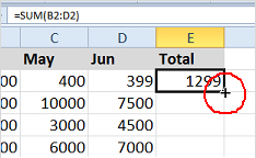
Filling down an Excel Formula in a column can be quickly achieved by positioning the cursor on the lower right corner of the cell and Double Clicking. The formula will repeat to the end of the data. For more ways
Double Click to Fill Down a Microsoft Excel Formula Read Post »