Applying Conditional Formatting to your data allows you to identify variances in a range of data with a quick glance, by highlighting the differences or trends that you specify. You can customize the process by creating your own rules to apply to selected data. To apply conditional formatting:
-
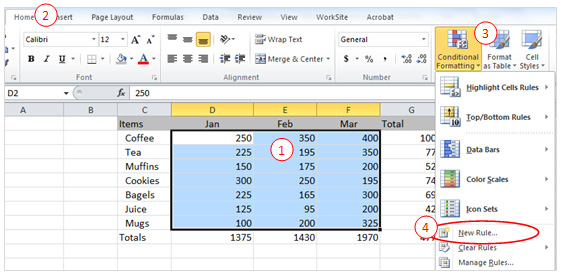
- Select the data range.
- Click the Home Tab.
- In the Styles Group, click Conditional Formatting.
- Select New Rule.
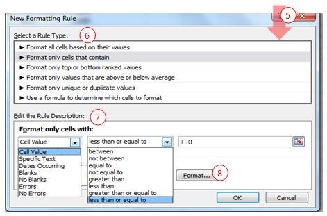
- The New Formatting Rule dialog box will open.
-
- Select a Rule Type: In this section select the type of criteria you want to use to determine formatting. In my example I am using Format only cells that contain.
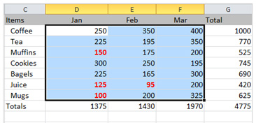
- Edit the Rule Description: In this section determine which criteria to apply to the selected area. In my example I will be formatting based on the Cell Value applying the condition less than or equal to 150.
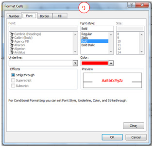
- Click the Format.
-
- The Format Cells dialog box appears. Select the formatting to be applied. In our example we will be changing the font color to red and making the text bold. You can also add a border or fill. Click OK twice.
-
- Formatting will then be applied.
-
- Repeat the process to apply additional formatting to a selected area.