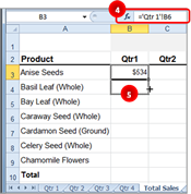
Excel allows you to reference or display values from other worksheets within a workbook. This is called a 3D reference. In the example below, we are going to pull the quarterly total from Sheet 1 to the Total Sales Sheet. Position the cursor in the cell where you want to display the number and press the equals sign (=). In our example the cursor is in cell B6 of the Total Sales worksheet. Excel 3d references Click on the sheet tab that has the number you want to display. (the Qtr 1 tab) Select the cell you want to display. Press Enter. This will move the cursor back to the original worksheet. Note: The formula bar will display the name of the sheet and the cell number. =’Qtr 1′!B6 Use the reference ‘Qtr 1′!B6 as you would any cell reference in a formula, so adding it would be =’Qtr 1’!B6 + b7. For more ways to make Excel work for you, take a training course from AdvantEdge Training & Consulting!

Here is a quick formula that calculates the current date each time you open your spreadsheet. Select a cell Type the following formula: <Today() Press Enter Excel Today’s Date Formula Now that cell will always display the current date and can be referenced in other formulas NOTE: you can also use the Now command if you would like to include the time as well: <Now() For more ways to make Excel work for you, take a training course from AdvantEdge Training & Consulting!

The F5 key is a great shortcut key in many of the Office programs for everything from navigating, inserting named ranges into formula, and starting a slide show.. F5 hotkey in Excel In Excel, pressing F5 will bring up the following dialog box listing past locations, name ranges, objects, worksheets, etc. Double click an item from the list to go to that location. F5 can also be used to access and insert name ranges in a formula. As you are typing in your formula, press F5 and then double click on your name range to be use. F5 hotkey in Word 2010 Pressing F5 in Word 2010 will launch the Find and Replace dialog box and in particular the Go To tab. From here you can navigate to various places in your document such as pages, sections, bookmarks, headings, etc. F5 hotkey in PowerPoint 2007 Pressing F5 from any place in PowerPoint will launch a slide show starting with the first slide. For more ways to make Excel work for you, take a training course from AdvantEdge Training & Consulting!

With Excel open, click the File Tab Click Options (towards the bottom of the menu) Click Advanced. In the Editing Options section, where it says “After pressing Enter, move the selection” change the direction to right Close out of the Excel Options For more ways to make Excel work for you, take a  training course from AdvantEdge Training & Consulting!

When you have a document that spans multiple pages, you might want your column titles/headers to be repeated on each page. Print Excel title columns and rows with these instructions. Click the Page Layout tab In the Page Setup group, click Print Titles In the Print titles section, place your mouse cursor in either the Rows or Columns fields (depending on which you want to repeat when printed) Click then drag-select the cells that contain the rows or column headers you want to repeat on each page For more ways to make Excel work for you, take a training course from AdvantEdge Training & Consulting!

By default, Excel shows the number of decimal places that can comfortably fit in a cell. If the cell is narrow, it might only fit one or two. A wider cell can fit many more. Sometimes, however, I want to show more or fewer decimal places. Making this change is easy to do. Right click on the cell you want to change, or select several different cells by first left clicking and dragging, then right clicking on the selected group. The first button with the arrow pointing left adds decimal places. The next button with the arrow pointing right, hides them. Choose whichever you like. Click on an empty part of the page to continue working on your spreadsheet. For more ways to make Excel work for you, take a training course from AdvantEdge Training & Consulting!

Identify cells and data with Excel name ranges. Excel name ranges make finding and identifying data easier. They can also be used in formulas in place of cell references. This makes formulas easier to understand and build. To use Excel name ranges in a formula: Select your desired cells Excel Name Box In the Name Box, above the row headings, type a name for the range (you cannot use spaces) then press Enter Go to any other spreadsheet Click the drop-down arrow in the Name Box and choose your named range from the list and note how it places you back into the spreadsheet with that range of cells selected Click in a cell and type a formula such as: =Sum( Excel Defined Names On the Formula tab in the Defined Names group, click the Use in Formula button and select the name of your range from the menu Type a close parentheses ) and press Enter View the formula in the formula bar and note that it does not use cell references but rather your named range For more ways to make Excel work for you, take a training course from AdvantEdge Training & Consulting!

Have you ever needed to reformat data so that the columns were the rows and the rows were the columns? Transposing in Excel is straightforward and easy. Select your data Copy your data with Control + C Click on the cell in which you want to transpose the data Right Click and choose Paste Special Check the Transpose box and click OK Find more ways Excel can make your life easier with a training course from AdvantEdge Training and Consulting.

Once you have created a macro, you can activate it in one click by adding it to the Quick Access Toolbar Click on the arrow at the end of the Quick Access toolbar and choose More Commands. This will open the Customize the Quick Access Toolbar dialog box. Choose Macros from the Choose commands from: drop-down list. Select your macro and click on Add. Click on Modify to rename the macro and select an icon for the macro. Click OK twice when finished. For more ways to make Excel work for you, take a training course from AdvantEdge Training & Consulting!

You can quickly sum a block of data (both Rows and Columns) in Excel with just one click. Start by selecting the data including the cells that will contain the SUM Formulas. (in our example Column E and Row 11) On the Home Tab in the Editing Section, click the SUM button. Excel will create a SUM function for each Row and Column. For more ways to make Excel work for you, take a training course from AdvantEdge Training & Consulting!