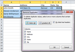
A common problem in processing data in Excel is handling duplicates or double entries. Excel has a few convenient tools for quickly making these changes. Simply eliminating duplicate entries in Excel After highlighting your chart of data, click on the Data tab and choose Remove Duplicates in the Data Tools group.The Remove Duplicates pop up window will be presented. First, check to see that the My data has headers box is checked. If you do have headers in your chart, then the header names should appear in the column section below. If not, then uncheck the box, and they should be labeled Column A, Column B, Column C, etc.Excel will identify duplicates that match all of the data entered. If you are only checking for duplicates in one column, and the contents of the other columns won’t matter, then make sure only that column header is checked. If you need to eliminate entries that are duplicated in 2 columns and the other columns won’t matter, just select those two. If everything needs to match, then make sure everything is checked.Once you’ve chosen your columns, click ok. The duplicate entries will be deleted. Manually sorting through duplicate entries in Excel In some cases, the data in the non-duplicated columns is important, and you might want to manually select which entry should be deleted. Excel makes this easy too.The first step will be to highlight all of the cells that are duplicated.Highlighting duplicate entries in ExcelFirst, Select the column or columns that contain duplicate entries be clicking on the letter at the top of the columns. Then, under the Home tab choose Conditional Formatting and Highlight Cells Rules and Duplicate Values. Choose one of the rules that includes a light red fill.Sort by cell color in ExcelThe next step will be to get all of the duplicate values to the top. If you’ve turned on filter then you can click on the drop down arrow by the header, choose Sort by color, and select light red or any other color you chose in the previous step.If filtering isn’t enabled, you’ll need to use custom sort. First highlight your data, then choose Sort from the Data tab. For Column, choose your column header, then change Sort on to Cell Color and for Order make Red go to the top.Either of these methods will bring the duplicate entries to the top. You might also want to add a sorting level that alphabetizes them first, since you’ll want each duplicate to be right next to each other.   Upgrade your Excel skills with training from AETC

Excel automatically converts numbers with 15 or more digits into scientific notation. In fact, when it simplifies the number it loses the rounded digits. They aren’t recoverable.As long as you don’t use numbers larger than a quadrillion, this isn’t a problem, but if you are using very long serial numbers or you really are calculating the distance to the sun in millimeters (roughly 149 quadrillion), then the full number format is better. Turning off Scientific notation in Excel Before typing your large number into the cell, change the cell format to Number from the drop down in the Number group of the Home tab. By default, Excel cells are General, which rounds numbers with more than 15 decimal places to scientific format. Number format doesn’t round it unless you tell it to.Change the format of the cell before typing your number. Rounded digits are unrecoverable. Turning on Scientific notation in Excel If you want scientific notation, then right click on the cell containing your number and choose Format Cells. Then, choose Scientific on the left and your desired number of decimal places.    For more ways to make Excel work for you, take a training course from AdvantEdge Training & Consulting!

How many days until the end of the year? How many days until the big meeting? Use this simple Excel countdown formula to find out.The DATEVALUE formula converts a date into a number in Microsoft Excel date-time code. This allows you to do simple math with days and time and create an Excel countdown formula.=DATEVALUE(“31-March-2012″)-TODAY()&” days until final numbers are due”The red section of the code does the math needed, and the blue section of the code adds “Days until Final numbers are due” to the cell. I included this to force Excel to use a number instead of printing the results in Date Time Format.If you don’t want a simple number instead, remove the blue section of the code. Then change the number format under the Home tab to “Number”.There are a few other applications for this beyond a simple Excel countdown formula too.     For more ways to make Excel work for you, take a training course from AdvantEdge Training & Consulting!

There a couple of ways to add page numbers to a Microsoft Excel worksheet.In the Page Layout tab, click on the Page Setup Additional Options button. Bring up the Header /Footer tab, and use the drop down menus to add the page numbers to either the header or footer. The Custom Header and Custom Footer buttons allow you to change the formatting. Click ok.The worksheet won’t look any different, but if you pull up a Print Preview, you’ll see your Excel page numbers added. Customizing Excel page numbers If you want to have more control over how your headers and footers look, use the page layout view.Under the View tab, click on Page Layout in the Workbook Views section. In this view, the phrase  “Click to add header” will be in a box just above your data. If you click on this box, the ribbon will show the Header & Footer Tools Design tab.You can manually type in information, or choose automatic fields like Page number, Number of Pages, date and time from the Header & Footer Elements.These icons insert code into the header and footer fields. So long as the code stays intact, you can type in content around the code. For example “This is page &[Page] of &[Pages]” will print as “This is page 5 of 6” (assuming it is page 5 of a 6 page document).To exit the Page Layout view, click on Normal under the View Tab. You’ll need to select a cell on the worksheet before you can choose a different view. For more ways to make Excel work for you, take a training course from AdvantEdge Training & Consulting!

If you have a large spreadsheet of information, you may often want to sort the information by more than one column. For example, what if you want to sort by date, but then sort by name within those dates?

Gridlines are the very lightly colored lines that surround each cell in a Microsoft Excel spreadsheet. Be default, they won’t print. Printing them is fairly easy though. To make Excel gridlines print Open your spreadsheet and click on the Page Layout tab. In the Sheet Options group, check the box for Print under Gridlines. To stop Excel gridlines from printing Open your spreadsheet and click on the Page Layout tab. Uncheck the box for Print under Gridlines in the Sheet Options group.Note, gridlines will only print in around cells with content. If you want to print blank cells with gridlines, select the area you want to print then click on Print Area in Page Setup and choose Set Print Area.   For more ways to make Excel work for you, take a training course from AdvantEdge Training & Consulting!

My Microsoft Excel Gridlines are no longer visible in the program. How do I get them back?There are 4 possible reasons that gridlines are no longer visible in Microsoft Excel. Reason for hidden Gridlines 1: They are turned off. Click on the View tab, then check the box for Gridlines in the Show group. Reason for hidden Gridlines 2: They are colored over. If the background color for a cell is white instead of no fill, then it will appear that the gridlines are missing. Select the cells that are missing the gridlines, or hit Control + A to select the entire workbook. Then, under the Home tab in the Font group change the color of the cells by clicking on the can of spilling paint and choosing no fill. Reason for hidden gridlines 3: The borders are colored white. Select the effected cells, or select everything with Control + A, then right click on the cells and choose Format Cells. Under the border tab, change the Color to Automatic. Reason for hidden gridlines 4: The gridlines have been colored white Click on the File tab. Then choose Options and Advanced. Scroll down to the Display options for this Worksheet section, and change the Gridline color to Black. Click OK.  For more ways to make Excel work for you, take a training course from AdvantEdge Training & Consulting!

Do you have a long spreadsheet that you need to print? Do you want to control which rows and columns are printed on which pages? You can use the page break settings to ensure it prints correctly.

3 Ways Excel can Betray You — We regularly hear harrowing stories of an accounting sheet gone wrong with an errant formula. These small mistakes are hard to catch and can lead to drastic consequences.If the total at the bottom of a chart doesn’t look quite right, it might be quite wrong. The following are common mistakes, leading to sums that don’t add up. Text Instead of Numbers — Just because a number is a number, doesn’t mean it’s a number. A “5” might mean the number 5 or it might be the text “5.” This issue happens most often when data is copied and pasted from Word or an email. Also, typing a dollar sign ($) or using a comma (1,000) (rather than using the cell formatting feature to insert these) may cause the number to be stored as text.Watch the alignment. If one number aligns to the left and the other aligns to the right, then the left aligning number is probably text. Excel might also point out the error to you with a small green triangle in the top left-hand corner of the formula cell. Not Including Enough Numbers — I was once told by a contractor that his company underbid a contract by tens of thousands of dollars because a sum formula didn’t include all of the correct cells.Excel warns you of this issue with a green triangle. Hover over the triangle and then click on the exclamation point to see the error message “Formula omits adjacent cells.” Either click on “Update formula to include omitted cells” or manually fix the formula.When adding more rows to a chart, confirm that any formulas include the new cells. If you insert a row between the last row and the “total” row, Excel may not automatically add the new row data to the formula.Avoid this by inserting rows in the middle of the data. Excel will then expand the formula to include the new row. Always double-check your formula and update as needed after adding new rows or columns. $b$16, Using Absolute Cell References Using the F4 key to make a cell reference absolute is a very useful trick when copying formulas, but be careful to use it correctly.Formulas using absolute cell references always refer to an exact cell, even if the formula is copied and pasted elsewhere in the document. Relative cell references, by contrast, refer to the cell relative to the position of the cell containing the formula — the default option if you don’t add the $$$ in your formula cell references.If copying a cell with a relative formula that adds the 3 cells above it, wherever you paste the formula, it will add the 3 cells above the new location. If the formula uses absolute references, however, it will still add the original 3 cells.Whether copying and pasting Relative or Absolute formulas, use the “Trace Precedents” option in the “Formula Auditing” group of the “Formulas” tab on the Ribbon to get a better look at exactly how the formulas are working.  For more ways to make Excel work for you, take a training course from AdvantEdge Training & Consulting!

When your data has been entered into Excel, you can use the built-in Filter tool on the Data Tab to narrow down what you are viewing based on criteria you set:On the Data tab, click the Filter button. (It’s a toggle button meaning: “one click on, one click off”) Click the arrow next to the column heading. You can pick the criteria to filter by, and narrow those results even further using the category filters, i.e., the date choices shown in the example.  Upgrade your Excel skills with training from AETC