AdvantEdge Blog | Consulting Professional Tips | Expert Advice
Excel

Excel Conditional Icons

Deciphering a spreadsheet is easier with Excel conditional icons, which visually communicate changes and differences in numbers with directional arrows, stop light colors, flags, and bars. In the example above, a simple sales report has been dressed up with Excel conditional icons. Inserting Excel conditional icons Select the cells in which you want to place your Excel conditional icons. Then, click on Conditional Formatting under the Home tab and choose Icons Sets. I selected the check mark indicators, but any set will do.We now need to edit the rules for the icons. Click again on Conditional Formatting, then Icon Sets and More Rules.This pop up window describes the rules for placing icons in the cells. You’ll need to set the values that will determine if the icon is green, yellow, or red. Excel can base this decision on exact numbers if you type numbers in the Value column or by a formula if you use the cell selector icon to choose a cell.In this example, I’m comparing each month’s sales against quota in cell e11, so I used the cell selector icon to choose that cell. If the value is greater than quota, the cell gets a check mark. If it is less then quota, it gets an X.By default, Excel offers three icons. I only want to use 2, so I changed the Icon for the final value to No Cell Icon. So if the sales figure is greater than or equal to 0, but less than quota, the cell will have an X excel conditional icon. If the sales figure is greater than quota, the cell will have a check mark.  For more ways to make Excel work for you, take a training course from AdvantEdge Training & Consulting!

Excel Conditional Icons Read Post »

Word

Word Overtype Mode

In Word 2003 you could press your insert key on your keyboard to either type over text or insert text. The default was to insert text, but you could quickly change that by using that key. Now in Office 2007 and 2010 the key doesn’t seem to work — how to you type over then without having to first select the text?There is a way to do this in the newer versions of Word, it is just not set up by default. Follow these steps to turn it on: From within Word, click on the File tab, then select Options Click on the Advanced option from the list In the Editing Options section, check the box next to Use the Insert key to control overtype mode . Click OK to exit the options Now you can use the Insert key to toggle the overtype mode on and off     Learn to make Word work for you with training from AETC.

Word Overtype Mode Read Post »

Excel

Finding Duplicates in Excel

A common problem in processing data in Excel is handling duplicates or double entries. Excel has a few convenient tools for quickly making these changes. Simply eliminating duplicate entries in Excel After highlighting your chart of data, click on the Data tab and choose Remove Duplicates in the Data Tools group.The Remove Duplicates pop up window will be presented. First, check to see that the My data has headers box is checked. If you do have headers in your chart, then the header names should appear in the column section below. If not, then uncheck the box, and they should be labeled Column A, Column B, Column C, etc.Excel will identify duplicates that match all of the data entered. If you are only checking for duplicates in one column, and the contents of the other columns won’t matter, then make sure only that column header is checked. If you need to eliminate entries that are duplicated in 2 columns and the other columns won’t matter, just select those two. If everything needs to match, then make sure everything is checked.Once you’ve chosen your columns, click ok. The duplicate entries will be deleted. Manually sorting through duplicate entries in Excel In some cases, the data in the non-duplicated columns is important, and you might want to manually select which entry should be deleted. Excel makes this easy too.The first step will be to highlight all of the cells that are duplicated.Highlighting duplicate entries in ExcelFirst, Select the column or columns that contain duplicate entries be clicking on the letter at the top of the columns. Then, under the Home tab choose Conditional Formatting and Highlight Cells Rules and Duplicate Values. Choose one of the rules that includes a light red fill.Sort by cell color in ExcelThe next step will be to get all of the duplicate values to the top. If you’ve turned on filter then you can click on the drop down arrow by the header, choose Sort by color, and select light red or any other color you chose in the previous step.If filtering isn’t enabled, you’ll need to use custom sort. First highlight your data, then choose Sort from the Data tab. For Column, choose your column header, then change Sort on to Cell Color and for Order make Red go to the top.Either of these methods will bring the duplicate entries to the top. You might also want to add a sorting level that alphabetizes them first, since you’ll want each duplicate to be right next to each other.   Upgrade your Excel skills with training from AETC

Finding Duplicates in Excel Read Post »

Excel

Scientific notation in Excel

Excel automatically converts numbers with 15 or more digits into scientific notation. In fact, when it simplifies the number it loses the rounded digits. They aren’t recoverable.As long as you don’t use numbers larger than a quadrillion, this isn’t a problem, but if you are using very long serial numbers or you really are calculating the distance to the sun in millimeters (roughly 149 quadrillion), then the full number format is better. Turning off Scientific notation in Excel Before typing your large number into the cell, change the cell format to Number from the drop down in the Number group of the Home tab. By default, Excel cells are General, which rounds numbers with more than 15 decimal places to scientific format. Number format doesn’t round it unless you tell it to.Change the format of the cell before typing your number. Rounded digits are unrecoverable. Turning on Scientific notation in Excel If you want scientific notation, then right click on the cell containing your number and choose Format Cells. Then, choose Scientific on the left and your desired number of decimal places.    For more ways to make Excel work for you, take a training course from AdvantEdge Training & Consulting!

Scientific notation in Excel Read Post »

Excel

Excel Countdown formula

How many days until the end of the year? How many days until the big meeting? Use this simple Excel countdown formula to find out.The DATEVALUE formula converts a date into a number in Microsoft Excel date-time code. This allows you to do simple math with days and time and create an Excel countdown formula.=DATEVALUE(“31-March-2012″)-TODAY()&” days until final numbers are due”The red section of the code does the math needed, and the blue section of the code adds “Days until Final numbers are due” to the cell. I included this to force Excel to use a number instead of printing the results in Date Time Format.If you don’t want a simple number instead, remove the blue section of the code. Then change the number format under the Home tab to “Number”.There are a few other applications for this beyond a simple Excel countdown formula too.     For more ways to make Excel work for you, take a training course from AdvantEdge Training & Consulting!

Excel Countdown formula Read Post »

Excel

Excel Page Numbers

There a couple of ways to add page numbers to a Microsoft Excel worksheet.In the Page Layout tab, click on the Page Setup Additional Options button. Bring up the Header /Footer tab, and use the drop down menus to add the page numbers to either the header or footer. The Custom Header and Custom Footer buttons allow you to change the formatting. Click ok.The worksheet won’t look any different, but if you pull up a Print Preview, you’ll see your Excel page numbers added. Customizing Excel page numbers If you want to have more control over how your headers and footers look, use the page layout view.Under the View tab, click on Page Layout in the Workbook Views section. In this view, the phrase  “Click to add header” will be in a box just above your data. If you click on this box, the ribbon will show the Header & Footer Tools Design tab.You can manually type in information, or choose automatic fields like Page number, Number of Pages, date and time from the Header & Footer Elements.These icons insert code into the header and footer fields. So long as the code stays intact, you can type in content around the code. For example “This is page &[Page] of &[Pages]” will print as “This is page 5 of 6” (assuming it is page 5 of a 6 page document).To exit the Page Layout view, click on Normal under the View Tab. You’ll need to select a cell on the worksheet before you can choose a different view. For more ways to make Excel work for you, take a training course from AdvantEdge Training & Consulting!

Excel Page Numbers Read Post »

Excel

Print Gridlines in Excel

Gridlines are the very lightly colored lines that surround each cell in a Microsoft Excel spreadsheet. Be default, they won’t print. Printing them is fairly easy though. To make Excel gridlines print Open your spreadsheet and click on the Page Layout tab. In the Sheet Options group, check the box for Print under Gridlines. To stop Excel gridlines from printing Open your spreadsheet and click on the Page Layout tab. Uncheck the box for Print under Gridlines in the Sheet Options group.Note, gridlines will only print in around cells with content. If you want to print blank cells with gridlines, select the area you want to print then click on Print Area in Page Setup and choose Set Print Area.   For more ways to make Excel work for you, take a training course from AdvantEdge Training & Consulting!

Print Gridlines in Excel Read Post »

Excel

Disappearing Excel Gridlines

My Microsoft Excel Gridlines are no longer visible in the program. How do I get them back?There are 4 possible reasons that gridlines are no longer visible in Microsoft Excel. Reason for hidden Gridlines 1: They are turned off. Click on the View tab, then check the box for Gridlines in the Show group. Reason for hidden Gridlines 2: They are colored over. If the background color for a cell is white instead of no fill, then it will appear that the gridlines are missing. Select the cells that are missing the gridlines, or hit Control + A to select the entire workbook. Then, under the Home tab in the Font group change the color of the cells by clicking on the can of spilling paint and choosing no fill. Reason for hidden gridlines 3: The borders are colored white. Select the effected cells, or select everything with Control + A, then right click on the cells and choose Format Cells. Under the border tab, change the Color to Automatic. Reason for hidden gridlines 4: The gridlines have been colored white Click on the File tab. Then choose Options and Advanced. Scroll down to the Display options for this Worksheet section, and change the Gridline color to Black. Click OK.  For more ways to make Excel work for you, take a training course from AdvantEdge Training & Consulting!

Disappearing Excel Gridlines Read Post »

If you have at least 5 people we can create a session just for you.  Or, you can contact us for a private session. Contact Us

Questions? Don't see what you need?

We can help!

Business Training Classes
AdvantEdge Training & Consulting, Inc.

Recent Posts

Subscribe to our Newsletter

Copyright AdvantEdge Training & Consulting

This site is protected by reCAPTCHA and the Google Privacy Policy and Terms of Service apply.

Scroll to Top