Microsoft Excel 2013 introduced a new feature that lets you differentiate data at a glance: Conditional formatting. This handy tool will apply colors to a cell’s font and background depending on the conditions you’ve set – for instance, if you want to highlight any cell that features a specific name or date, or differentiate high, medium and low numerical values. Follow these directions to set up your own conditional formatting in a few simple steps.
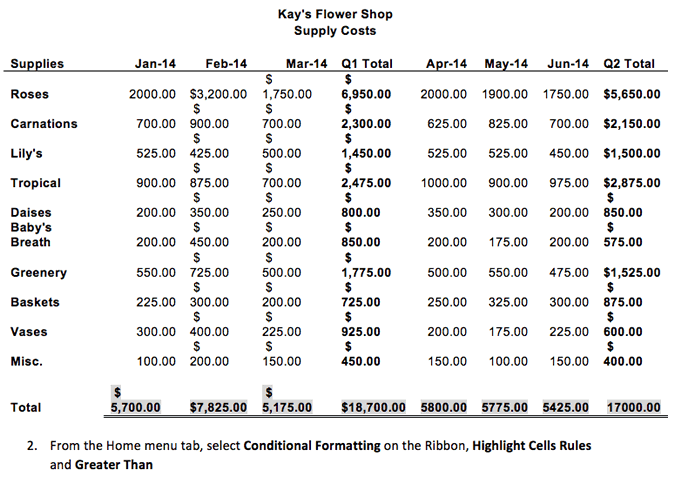
1. Select the cells you want to format.

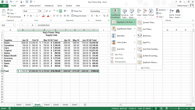
2. From the Home menu tab, select Conditional Formatting on the Ribbon, Highlight Cells Rules and Greater Than

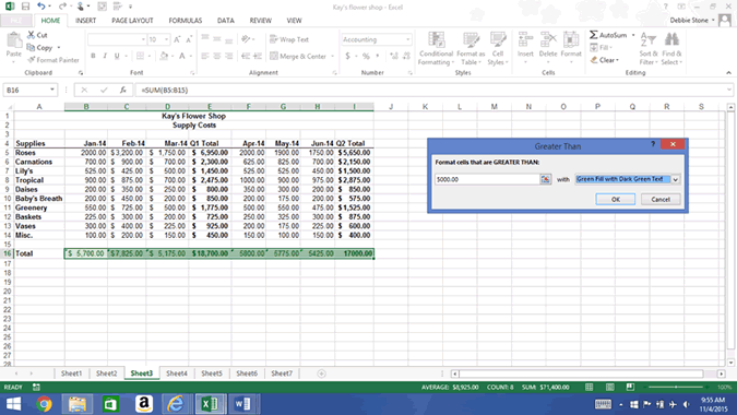
3. In the Greater Than box, type your threshold amount that you want the cell amounts to be reflected by the color in the “with” box. In the example below, we want any amount greater than 5000.00 to have a green background with green text.

Your business training experts!


